Overview
This year, the aim of our project is to create a novel biomaterial by engineering Ultrabithorax protein. We utilized models in our engineering cycles and further applied them to future implementation. Prior to engineering cycle 1, we used the protein structure prediction model to predict Ubx protein structure to obtain better insights associated with Ubx protein properties. Yet, the protein expression of the Ubx is below expectation. In engineering cycle 2, we further narrowed down to dityrosine-containing domains among Ubx sequences, as dityrosine cross-linkings are evidenced to drive the assembly of proteins and peptides. Thus binding region prediction model was built to precisely predict the formation of dityrosine cross-linking among Ubx sequences. In engineering cycle 3, in the functional test, we developed a tyrosine binding model to predict the best circumstance for the formation of dityrosine bonds. Eventually, we built a protein mixing model for future implementation in bioprinting a scaffold for tissue engineering by analyzing the relationship between protein concentrations and the output color.

Protein Structure Prediction
The properties of Ubx are determined by its protein structure. We used Alphafold2 to conduct our protein structure prediction, as we were not able to obtain the Ubx protein PDB database. With an atomic scale accuracy algorithm, Alphafold2 is vastly more accurate than other competing methods. In our project, we used the collab version of Alphafold2, whose open-source program can now be executed on google collab
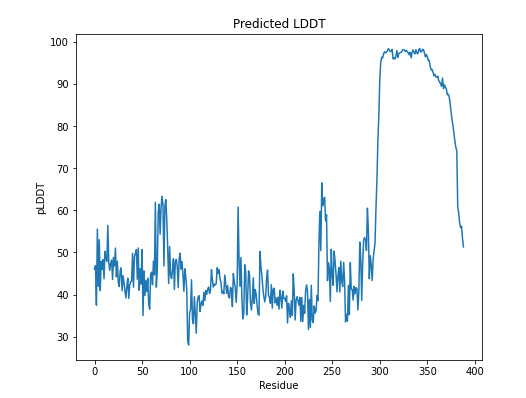
There are two important outputs that represent the confidence score of the prediction result. First, pLDDT (predicted IDDT-Cα) is a per-residue measure of local confidence on a scale from 0-100. The region with low pLDDT may be associated with either unstructured in isolation or intrinsically disordered. The region with high pLDDT may be a structured domain.1
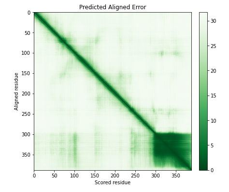
To assess confidence in the domain packing and large-scale topology of the protein, we had our second output, PAE (predicted aligned error). In the graph below, the color demonstrates the confidence score in relative domain positions. The color at (x, y) corresponds to the expected distance error in the residue x's position, and the prediction and true structure are aligned on residue y. Low PAE (dark green) means Alphafold is confident about the relative domain positions. On the other hand, high PAE (light green) means Alphafold is less confident about the relative domain positions.2
Conclusion
Prior to engineering cycle 1, we can presume that Ubx is disordered between 1 - 281 residue and has a fixed structure between 281 - 389, according to the results above.
Binding Region Prediction
In engineering cycle 1, the production of Ubx is below expectation. Thus, the binding region prediction model was built to precisely predict the formation of dityrosine cross-linking among Ubx sequences for the purpose of further narrowing down to dityrosine-containing domains among Ubx sequences, as dityrosine cross-linkings are evidenced to drive the assembly of proteins and peptides.
In step 1, we used the ANCHOR algorithm to predict the region among Ubx sequences that demonstrate better binding. In step 2, we utilized the result from step 1 and further built a selection model precisely to predict the exact formation of dityrosine cross-linking among the possible binding sites.
The basic concept of ANCHOR algorithm is to input an amino acid sequence and predict protein binding regions that are disordered in isolation but can undergo disorder-to-order transition upon binding.

3
After the analytics of the ANCHOR algorithm, we further utilize the results and build a selection model to analyze the distance between lysine and tyrosine. The selection model has further specified the binding probability of tyrosine.
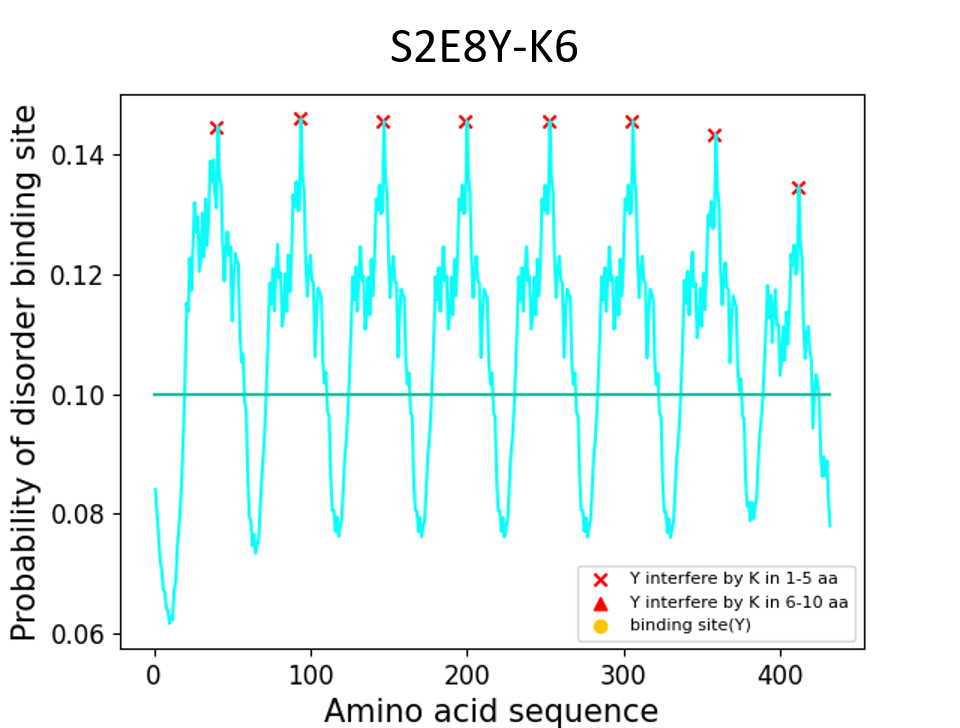
According to the research, we understand the prerequisites for crosslinking among tyrosines. To be more clear, crosslinking will be affected by positively charged lysines and decreased π–π interactions among tyrosines. Moreover, lysines can also reduce the rate of tyrosine formation and decrease the number of dityrosine bonds. There are three cases for different distances between lysine and tyrosine.4
First, when the distance between lysine and tyrosine is more than 10 residues, the positive charge of lysine won't affect the tyrosine residue.
Second, when the distance between lysine and tyrosine is between 6 to 10 residues, the positive charge of lysine will affect tyrosine but will not affect the performance of crosslinking.
Third, when the distance between lysine and tyrosine is equal or under 5 residues, the positive charge of lysine will affect tyrosine. Under this condition, tyrosines will not crosslink.
Based on the research, we generated three testing data to validate our model.5
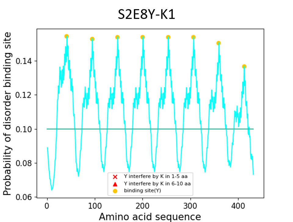
S2E8Y-K1 (silk-elastin-like polymers (SELPs) amino acids sequence)
MAMGGGA - [(GAGAGS)2 K(GVGVP) (GVGVP) (GVGVP) (GVGVP) (GYGVP) (GVGVP)3]8 - Gwhich K (lysine) is 21 (>10) residue far from Y (tyrosine)
Results
S2E8Y-K3
MAMGGGA - [(GAGAGS)2(GVGVP) (GVGVP)(GVGVP)K(GVGVP) (GYGVP) (GVGVP)3]8 - Gwhich K (lysine) is 7 residue far from Y (tyrosine)
Results

S2E8Y-K6
MAMGGGA - [(GAGAGS)2(GVGVP) (GVGVP) (GVGVP) (GVGVP) (GYGVP)K(GVGVP)3]8 - Gwhich K (lysine) is 4 residues close to Y (tyrosine)
Results
Finally, to precisely predict the exact formation of dityrosine cross-linking among the possible binding sites in Ubx, we input our baseline value as 0.6, which is considered to be more rigorous. The results of our Ubx sequence in our model package are in the graph below.
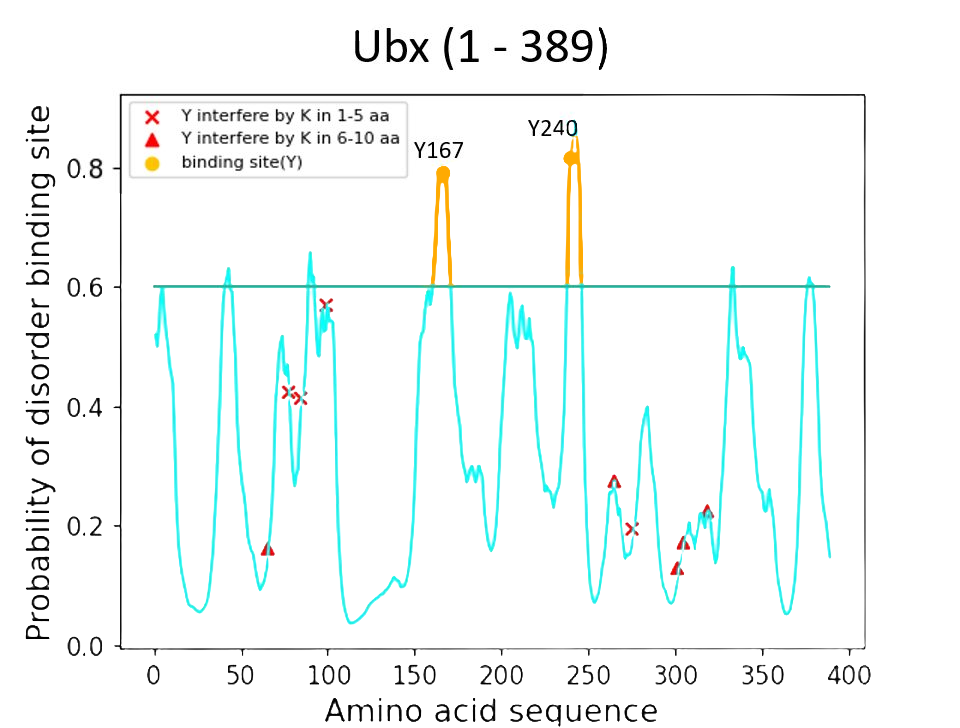
Conclusion
According to the result of the ANCHOR algorithm and the model we built, Y167 region and Y240 of the Ubx showed the best probability of forming dityrosine cross-linking. Thus, we further engineer Y167 and Y240 with functional protein mRFP in our engineering cycle 3.
Validation
The result of the binding prediction model has led us to select Y167 and Y240 and engineer them with mRFP in our engineering cycle 3 to test the properties of Ubx - self-assembly. By observing self-cross-linking in our functional test, we could validate the correctness of our prediction.
For more details see our Results
Tyrosine Binding Model
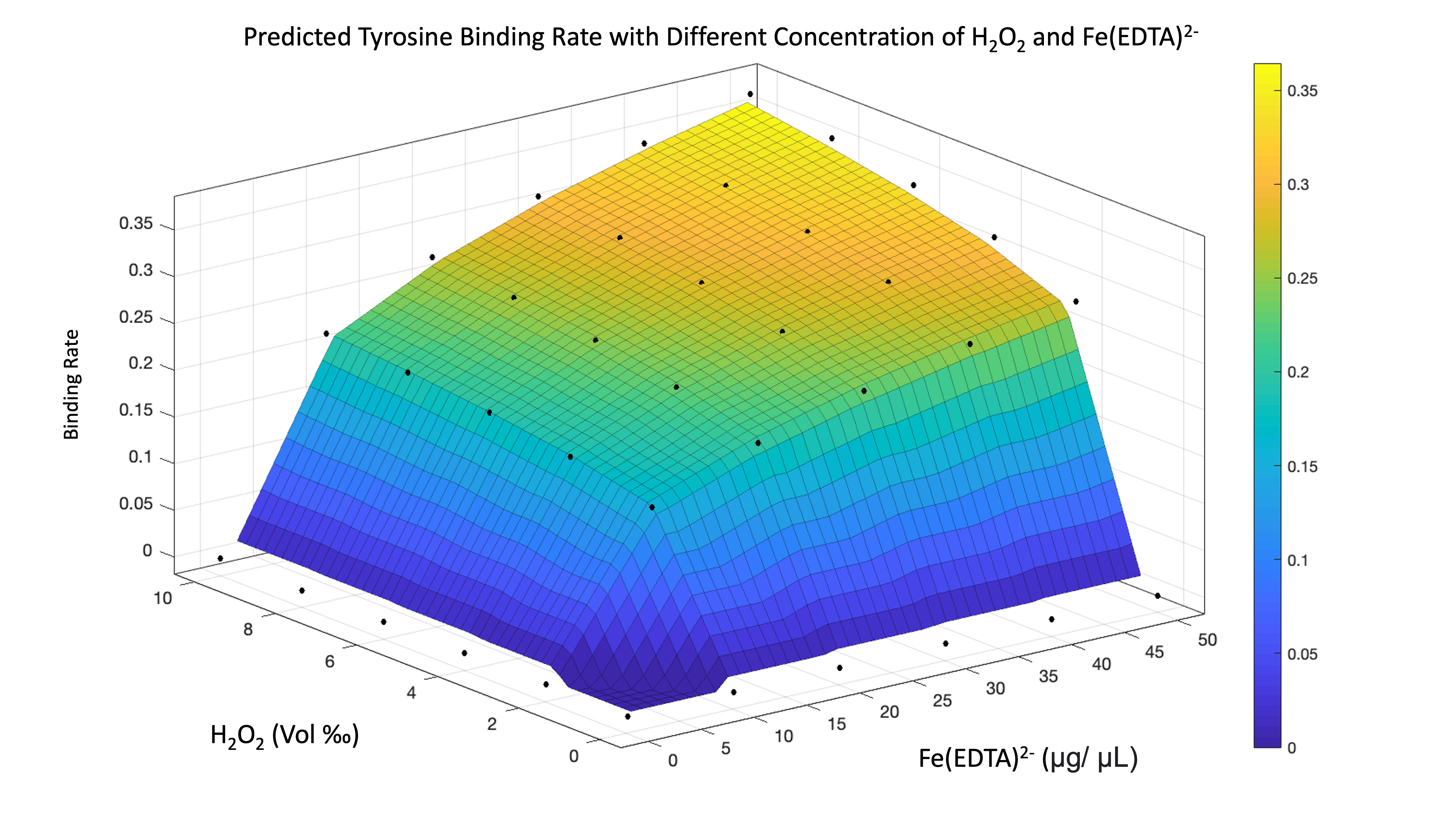
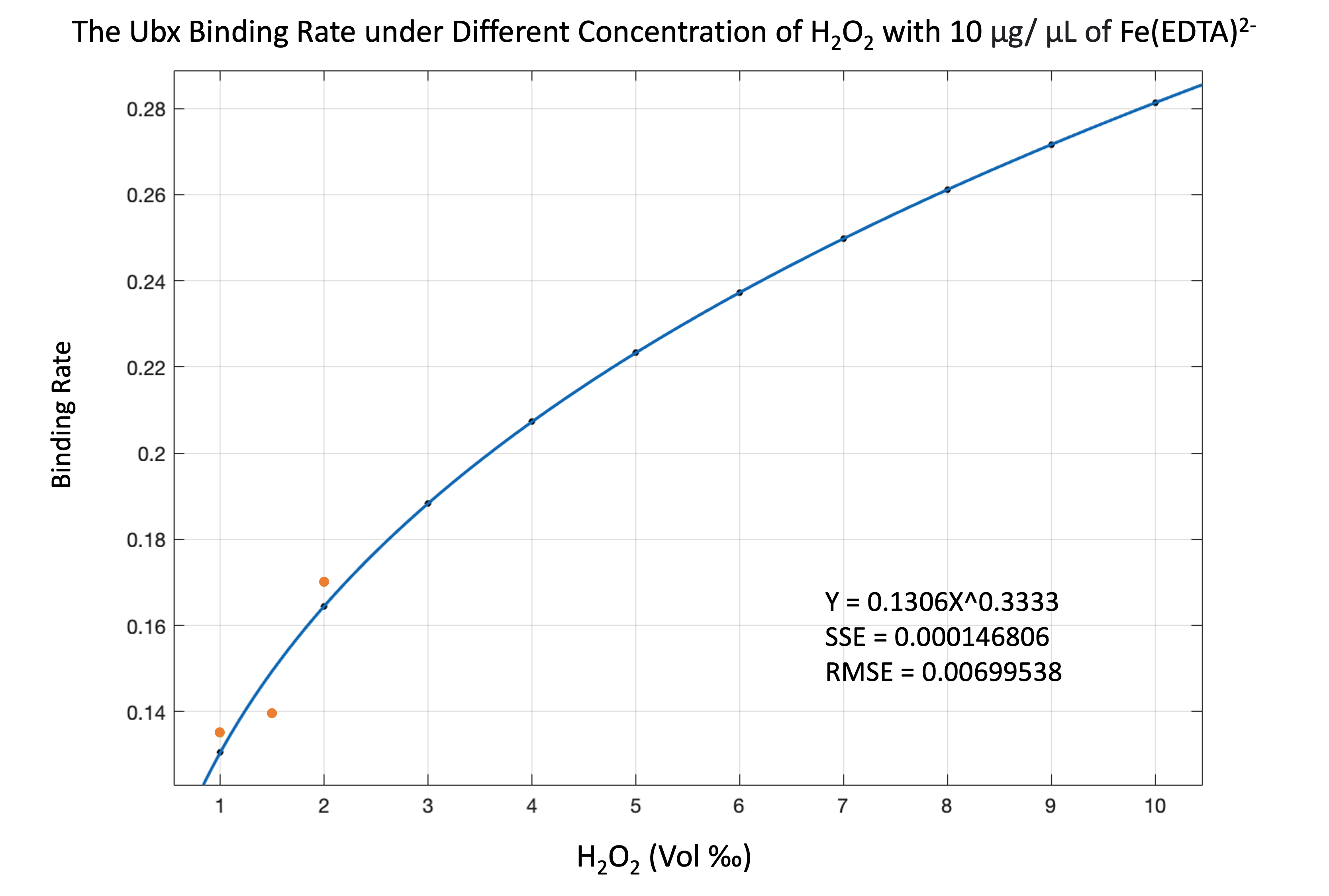
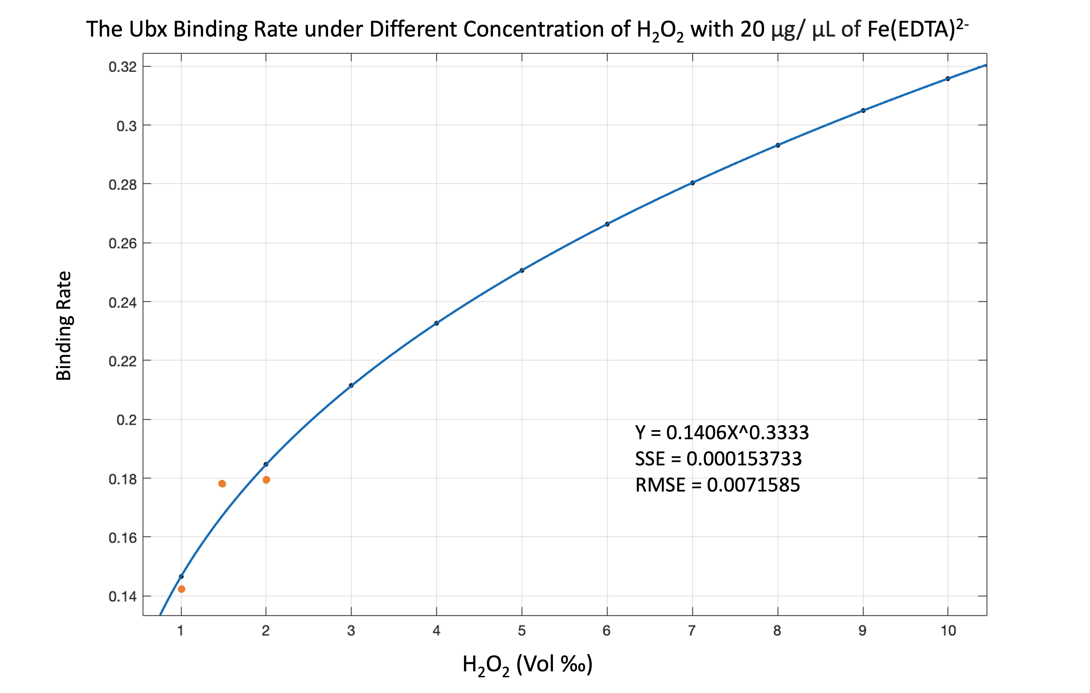
With the Y167 and Y240 tyrosines, the functional proteins can assemble while the dityrosine bonds are forming. While our wet lab group was trying to conduct functional tests, we wanted to simulate the assembly result of our product. The factors that affect the formation of bonds are related to the concentration of H2O2, Fe(EDTA)2-, and our functional protein. Hence, we want to simulate the binding rate of tyrosine under different portions of H2O2 and Fe(EDTA)2-.
Simulation
To make tyrosine bond together, we selected H2O2 and Fe(EDTA)2- to provoke it. We aimed to let hydroxyl radicals oxidize the tyrosine; then, they would form the dityrosine bonds. The first step is the Fe2+ separated from Fe(EDTA)2-. See equation 1. We assume the equilibrium constant as K1
\begin{equation} \begin{align*} Fe(EDTA)^{2-}\rightleftharpoons Fe^{2+} + EDTA^{4-} \quad K_{1} = 4.7863\times 10^{-15} \\ \end{align*} \end{equation}
The next step is H2O2 reduced to hydroxyl radical with the iron(ii) becoming iron(iii). See equation 2. In this step, we assume the equilibrium constant as K2.
\begin{equation} \begin{align*} Fe^{2+} + H_{2}O_{2}\rightleftharpoons Fe^{3+} + OH^{-} + \cdot OH \quad K_{2} = 5.7\times 10^{2} \\ \end{align*} \end{equation}
Last, the hydroxyl radical will oxidize the tyrosine. Unstabled oxidized tyrosines will form dityrosine bonds. Because of the high reduction potentials of hydroxyl radical (1.8–2.7 V vs. NHE), we consider the equation as an irreversible equation.6
See equation 3.
\begin{equation} \begin{align*} 2 \cdot OH + 2\,Tyrosine \rightarrow Dityrosine + 2H_{2}O \\ \end{align*} \end{equation}
With equation 1, we can get [Fe2+] as below
\begin{equation} \begin{align*} \left [ Fe^{2+} \right ] = \sqrt[2]{K_{1}\cdot \left [ Fe(EDTA) \right ]} \\ \end{align*} \end{equation}
with equation 2 and 4, we obtain [.OH] as
\begin{equation} \begin{align*} \left [ \cdot OH \right ] = \sqrt[3]{K_{2}\cdot \left [ EDTA^{4-} \right ]\cdot \sqrt[2]{K_{1}\cdot \left [ Fe(EDTA) \right ]}} \\ \end{align*} \end{equation}
| Parameter | Name | Value | Referece |
|---|---|---|---|
| K1 | Equilibrium constant of equation 1 | 4.7863*10-15 | 7 |
| K2 | Equilibrium constant of equation 2 | 5.7*102 | 8 |
| [Protein] | Protein concentration at 12 hr | 0.014330848 M |
By analyzing the equation, we found that if the concentration of protein is more than hydroxyl radical, the combining rate is the fraction of protein concentration to hydroxyl radical concentration. If the concentration of protein is less than or equal to hydroxyl radical, we consider the combination rate to be 1.
\begin{equation} \begin{align*} Binding\,Rate = 1 \quad if \left [ \cdot OH \right ] \geq \left [ Protein \right ] \\ Binding\,Rate = \frac{\left [ \cdot OH \right ]}{\left [ Protein \right ]} \quad if \left [ \cdot OH \right ] \leq \left [ Protein \right ] \\ \end{align*} \end{equation}
Results
By using the equation, we can see the result of simulating binding rate as figure 11-13.
Protein Mixing Model
A Ubx scaffold plays an important role in 3D bioprinting. To improve the accuracy and quality of 3D bioprinting, we analyzed how different concentrations of protein affect stem-cell differentiation. In 3D bioprinting, functional proteins are covered on the Ubx scaffold. Every organ or cell corresponds to different kinds of stem-cell differentiation, which means that there exists a unique combination of functional proteins inducing cell differentiation. In order to analyze the relationship between the configuration of protein’s concentration and the type of the ultimate organ, we decided to use RFP, GFP, and BFP to simulate the combination of proteins. Different proportions of RFP, GFP, and BFP lead to different colors and wavelengths, which leads to different RGB values. In this way, we can clearly understand the concentration of each protein on the scaffold by analyzing the RGB values of the color through our protein mixing model. Conversely, we are also able to predict the final color, which is mixed by the given RFP, GFP, and BFP, on a specific unit area of the scaffold.
Output Color Simulation
Besides wavelength, RGB values are another way to represent a color. This model shows that different intensities of red, green, and blue lead to different colors.
rgb(122.5, 122.5, 122.5)
Color Combination Simulation
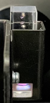
The ratio of two different proteins determines the functionality of the cell after cell differentiation. We decided to use colors to represent what type the protein is. The color on the left represents type A protein. The color on the right represents type B protein. This simulation shows that, on the Ubx scaffold, different ratios of protein can mix up to different colors, which is displayed in the middle area. Users can freely change the ratio between two kinds of protein by adjusting the rod.
Scaffold Simulation
Every function of an organ has its own organization of protein. Different protein concentrations on the scaffold will lead to different results. Thus, knowing how the final product looks under fluorescence is crucial in 3D bioprinting. We designed a specific combination of protein concentration in each area of the coral-like scaffold, which is represented by pixels, and simulated the color combination in the timescale of 0 to 14 hours.9
Step One: RGB Extraction
We designed a draft with a given width and height. After RGB values of pixels are extracted in rows and columns (code) by image J, we converted them into fluorescent RGB values. After measuring the maximum wavelength by the Elisa reader and converting them to RGB values, we input (255,179,0) as the RGB values of RFP (E1010) and (166, 255, 0) as the RGB values of GFP (E0040).10, 11
The following formula is our protein mixing model (Formula 4).12
The letter 'r' means the result color. A means the opacity.13
A1 means the opacity of the first color. A2 means the opacity of the second color. r.R, r.G, and r.B, respectively, represent the red, green, and blue values of the result color. After conversion, the converted RGB values need to be adjusted according to the intensity measured by our experiment. The following formula gives a clearer understanding of the relationship between RGB values and perceived luminance and hence proves that RGB values represent luminance intensity.14
\begin{equation} \begin{align*} r.A = 1 - (1 - A2)\cdot (1 - A1) \\ r.R = R2\cdot \frac{A2}{r.A} - R1\cdot A1\cdot \frac{1-A1}{r.A} \\ r.G = G2\cdot \frac{A2}{r.A} - G1\cdot A1\cdot \frac{1-A1}{r.A} \\ r.B = B2\cdot \frac{A2}{r.A} - B1\cdot A1\cdot \frac{1-A1}{r.A} \\ \end{align*} \end{equation}
Luminance is a linear measure of light. Before being converted to luminance, all RGB values are converted to decimal 0 - 1.0. V’ is the encoded gamma RGB. If V’ is larger than 0.04045, it requires a power curve of approximately V^2.2. (Formula 1) To find the luminance, we applied the standard coefficients for linear RGB values. In contrast, perceived lightness is nonlinear, as in human perception. We need to input the luminance into the function (Formula 3) to get the perceptual luminance.
\begin{equation} \begin{align*} V_{linear} = \left\{\begin{matrix} \frac{V^{'}}{12.92} & V^{'}\leq 0.04045\\ \left ( \frac{V^{'} + 0.055}{1.055} \right )^{2.4} & V^{'} \geq 0.04045 \end{matrix}\right. \end{align*} \end{equation}
\begin{equation} \begin{align*} Y = R_{lin}\cdot 0.2126 + G_{lin}\cdot 0.7152 + B_{lin}\cdot 0.0722 \end{align*} \end{equation}
Step Two: RGB Adjustment
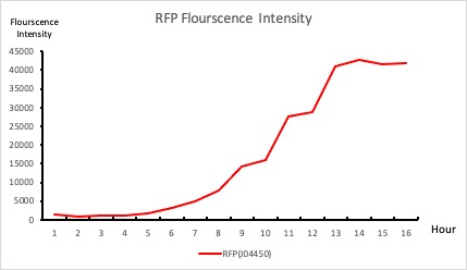
We adjust the intensity of RGB values respectively according to the intensity-to-time relationship acquired from GFP (E0040), RFP (E1010) experiments. However, BFP (K1033902) from the kit was not transformed successfully, and there are not any data regarding the intensity-to-time relationship of the BFP(K1033902). We decided to retain every blue value without converting it into the RGB values of BFP.
Step Three: Scaffold Simulation
The adjusted RGB values of each pixel are imported into the numpy array written in Python (code). Pixels are arranged in the form of the given specific height and width. Finally, we got the final scaffold simulation saved as png files. The following eight pictures are the results.
Experiment Verification for Protein Mixing Model
The following picture (Figure 14) shows different combinations of GFP (E0040) and RFP (E1010). We used image J to measure the RGB values. The mean RGB values of pure RFP are (254.72,140.96,43.39). The mean RGB value of pure GFP is (227.33,210.12,52.10). If the combination of RFP and GFP is 5 to 3, the mean RGB value is (250.25,170.85,48.67). The amount of error of red, green, and blue values are 3%, 2%, and 3%, which is acceptable. We speculated that the error was caused by the color of the shield. However, this verification still proves that our protein mixing model is trustworthy.

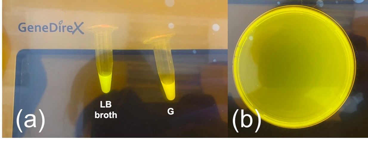
The intensity-to-time relationship of the GFP (E0040) measured by our experiment does not have a distinctive slope(Figure 16). The reason is that the color of the GFP (E0040) and the color of the LB broth are similar (Figure 17(a)). However, we decided not to remove the intensity provided by the LB broth, because the color of the LB broth and the color of the plate, which consists of LB Agar, are similar too (Figure 17(b)).


Experiment Verification for Color Mixing Model
The intensity-to-time relationship of the GFP (E0040) measured by our experiment does not have a distinctive slope(Figure 16). The reason is that the color of the GFP (E0040) and the color of the LB broth are similar (Figure 17(a)). However, we decided not to remove the intensity provided by the LB broth because the color of the LB broth and the color of the plate, which consists of LB Agar, are similar too (Figure 17(b)).
The following picture (Figure 7) shows different combinations of GFP (E0040) and RFP (E1010). We used image J to measure the RGB values. The mean RGB values of pure RFP are (254.72,140.96,43.39). The mean RGB value of pure GFP is (227.33,210.12,52.10). If the combination of RFP and GFP is 5 to 3, the mean RGB value is (250.25,170.85,48.67). The amount of error of red, green, and blue values are 3%, 2%, and 3%, which is acceptable. We speculated that the error was caused by the color of the shield. However, this verification still proves that our color mixing model is trustworthy.
Reference
- Mariani, V., Biasini, M., Barbato, A., & Schwede, T. (2013). lDDT: a local superposition-free score for comparing protein structures and models using distance difference tests. Bioinformatics, 29(21), 2722-2728.
- Jumper, J., Evans, R., Pritzel, A. et al. Highly accurate protein structure prediction with AlphaFold. Nature 596, 583–589 (2021).
- Dosztányi, Z., Mészáros, B., & Simon, I. (2009). ANCHOR: a web server for predicting protein binding regions in disordered proteins. Bioinformatics (Oxford, England), 25(20), 2745–2746.
- Mészáros B, Simon I, Dosztányi Z (2009) Prediction of Protein Binding Regions in Disordered Proteins. PLOS Computational Biology 5(5): e1000376.
- Constancio Gonzalez-Obeso, Fredrik G. Backlund, and David L. Kaplan Biomacromolecules 2022 23 (3), 760-765 DOI: 10.1021/acs.biomac.1c01192
- Hangasky, J. A., Detomasi, T. C., Lemon, C. M., & Marletta, M. A. (2020, August 3). Glycosidic bond oxidation: The structure, function, and mechanism of polysaccharide monooxygenases. Comprehensive Natural Products III (Third Edition). Retrieved October 12, 2022
- Wang, Sheng-Wei & Liu, Chen-Wuing & Lu, Kuang-Liang & Chang, Yu-Piao & Chang, Ta-Wei. (2011). Distribution of Inorganic As Species in Groundwater Samples with the Presence of Fe. Water Quality, Exposure and Health. 2. 181-192. 10.1007/s12403-010-0036-1.
- https://www.sciencedirect.com/science/article/pii/B9780128032695000012
- The colorful, dark, dynamic art of life: 2015 BioArt winners
- https://stackoverflow.com/questions/56415924/convert-javascript-hex-rgb-color-to-wavelength-and-vice-versa
- https://www.thermofisher.com/tw/zt/home/life-science/cell-analysis/cell-analysis-learning-center/molecular-probes-school-of-fluorescence/fluorescence-basics/fluorescence-fundamentals/light-spectrum-fluorescence.html
- https://itecnote.com/tecnote/r-algorithm-for-additive-color-mixing-for-rgb-values/
- https://www.w3schools.com/css/css3_colors.asp
- https://stackoverflow.com/questions/596216/formula-to-determine-perceived-brightness-of-rgb-color