ViralessMe
Problem
Calibration
After the optic fiber sensor has been functionalized, it has to be calibrated and tested in sucrose solutions with different concentrations, to see whether calibration went well or not. If the calibration was successful, then the optic fiber readings would correlate with the concentration change of sucrose solution, otherwise there wouldn't be significant correlation indicating that the sensor is not viable for work.
Whether the sensor was calibrated successfully or not is checked by running the readings through matlab script which compares the optic fiber sensor readings with predetermined refractive index values. Predetermined refractive index values are just the expected refractive indexes which certain sucrose concentrations should have. In a nutshell, when, say sucrose concentration is 1 arbitrary unit, then the light emitted from optic fiber should refract in a certain manner (most likely slower), so that the medium is expected to have a refractive index of 1.5 arbitrary units.
Should our product be in a lab or field, matlab script for calibration evaluation has to be adapted for the readings number and type each time. Our product target audience is not expected to have sufficient matlab experience to modify the script accordingly every time they want to check whether the sensor is calibrated. More to that, calibration checking should be done after each functionalization - which would occur frequently - hence making script modifications an inconvenient and time consuming process.
Experiment
If the sensor is properly calibrated, it can be tested in the media containing possible antigens. For that, the sensor is connected to OFDR (apparatus to read optical fiber responses) and immersed into solutions with different concentrations of antigens. The responses of optical fiber biosensors at different concentrations of antigens are saved as text files:

FIgure 1. Experiment data format
To analyze the results, another matlab script is used. It makes a scatterplot from the text files, where each point represents one reading. The y-axis of the scatterplot is the amplitude or return loss measured in dB by the sensor and the x-axis is sample concentrations. If the the initial samples do not contain antigens, then all the points should have roughly the same amplitude, since the amplitude would change if the antigens would bind to the antibodies located on the sensor:

Figure 2. Graph of sample containing antigens.
Otherwise, if the scatterplot displays some kind of relationship between the changing concentrations and amplitude, then the sample is said to contain antigens.
Just like with the calibration script, the experiment script also has to be modified based on the different parameters.
Solution
In order to make the data analysis and calibration evaluation processes more convenient, quicker, and user-friendly, we developed a software which unites both scripts, and automatizes the process of matlab script modification.
Principle of work
The user must first choose his purpose: calibration evaluation or the analysis of experimental data.

Based on the user choice, the python script opens the corresponding matlab script, and changes lines indicating the number of points, x-axis, y-axis, concentrations inside the matlab script. After the script has been modified accordingly, the user can press the “Analyze” button and the python program will return the graph and calibration information (if calibration is chosen):

Figure 3. Results for optic fiber's response analysis
Figure 4. Results for optic fiber calibration
The software can run the experiment analysis matlab script with a maximum of 14 readings (otherwise it won't fit within the x-axis). As per the calibration readings, it can only work with exactly 6 readings because of calibration protocol restrictions.
After the script is run, it can perform analysis multiple times without the need to execute the script again. In other words, once the user starts the script, they can first run the calibration evaluation, then within the execution run the experimental data analysis.
To create convenient and easy-to-use interface the tkinter library is used:
To run the matlab scripts directly inside python, the maltab.engine is used. It is important to note that in order for the matlab.engine library to run, the user has to have pre-installed matlab:

Note
In the experimental data analysis, the input data have to be in the format demonstrated in figure 2, otherwise it is impossible to parse the files with random names.
For calibration evaluation, following data naming conventions should be used:

Figure 5. Naming of files for calibration
dnaTurner
dnaTurner
Once we have aptamer sequences ready, there are few advantages to knowing its 3D structure. Besides observing how the nucleotide sequences are folding, it gives an edge to test how well they bind their target proteins via in-silico model simulations.
DNA aptamers are usually no ordinary DNA molecules, but single-stranded ones, and researching the internet, we did not find tools to predict the 3D structure of single-stranded DNAs. A usual way to predict 3D structures of ssDNA molecules is to follow a sequence of steps using multiple tools on the internet (see design page for more information (link to the design page)).
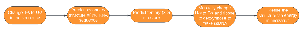
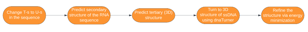
However, it includes a step where one has to do a laborious job of modifying the .pdb files of RNA molecules to change uracil to thymine, and ribose to deoxyribose, in order to turn the RNA molecule into a ssDNA molecule. So we created a program dnaTurner that does this laborious job automatically, and it is available on gitlab. Therefore the sequence of steps to predict the 3D structure of single-stranded DNA molecules becomes:
The software was inspired by iGEM INSA-Lyon 2016 team, who made a software for similar purposes that included dnaTurner’s functionality, but used outdated programs so that it is hard to use now.
Principle of work
dnaTurner reads the pdb files of RNA molecules, and turns an Uracil nucleotide into Thymine by changing the corresponding hydrogen atom (H) into a methyl group (CH3), and turns a ribose into deoxyribose by altering the corresponding hydroxyl group (OH) into hydrogen atom (H) in all nucleotides, so overall, the program turns the RNA sequence back into the original DNA sequence, and the resulting file is the 3D structure of the single-stranded DNA molecule.
Usage
Let’s try to predict the 3D structure of a ssDNA molecule using dnaTurner. One of the aptamers we designed in scope of our project is the following DNA aptamer for a vaccinia virus protein L1.
ATCGTGAGGAAGCGGCGGGA
The first step is to change its Thymine nucleotides into Uracil in order to make it a RNA sequence:
AUCGUGAGGAAGCGGCGGGA
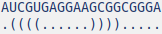
Then make its secondary structure. One way to do it is via internet tools such as Mfold. A predicted secondary structure of the RNA sequence above shown below:
The next step is to use the secondary structure to predict the 3D structure of the RNA sequence. One can do it using available web tools; we used RNAComposer. The resulting 3D structure of the RNA sequence is as follows:
The next step is to turn this 3D structure into the 3D structure of the original DNA aptamer sequence using dnaTurner. For this, one needs to execute the dnaTurner.py file:
python3 dnaTurner.py -i L1_aptamer.pdb -n L1_aptamer
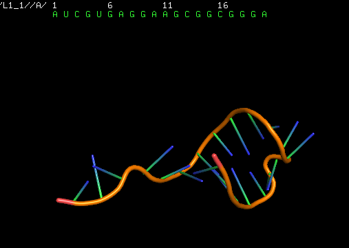
And it is highly recommended to run the resulting .pdb file through the energy minimization process, to refine the shape of the modified 3D structure in correspondence with the applied changes. We used QRNAS software for this purpose. The resulting 3D structure of the single-stranded DNA aptamer is shown below:
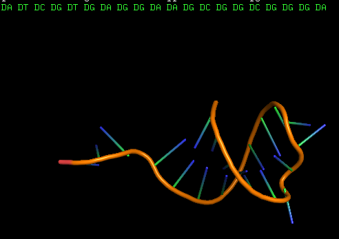
In comparison with the 3D structure of the intermediate RNA sequence, it can be noticed that the nucleotides have changed to DNA nucleotides, along with slight changes in the 3D shape of the molecule due to turning it into a DNA molecule.
References
-
Oliveira, R., Pinho, E., Sousa, A. L., Dias, Ó., Azevedo, N. F., & Almeida, C. (2022). Modelling aptamers with nucleic acid mimics (NAM): From sequence to three-dimensional docking. Plos one, 17(3), e0264701, https://doi.org/10.1371/journal.pone.0264701.
-
Zuker M. Mfold web server for nucleic acid folding and hybridization prediction. Nucleic Acids Res. 2003;31: 3406–3415. pmid:12824337
-
Antczak, M., Popenda, M., Zok, T., Sarzynska, J., Ratajczak, T., Tomczyk, K., Adamiak, R.W., Szachniuk, M. New functionality of RNAComposer: an application to shape the axis of miR160 precursor structure, Acta Biochimica Polonica, 2016, 63(4):737-744 (doi:10.18388/abp.2016_1329).
-
Popenda, M., Szachniuk, M., Antczak, M., Purzycka, K.J., Lukasiak, P., Bartol, N., Blazewicz, J., Adamiak, R.W. Automated 3D structure composition for large RNAs, Nucleic Acids Research, 2012, 40(14):e112 (doi:10.1093/nar/gks339).
MAWS Guide
In the process of our work with aptamers, we have met with several iGEM teams and found out that they are struggling with using MAWS to make aptamer sequences, and since we were able to figure out how to use MAWS to design aptamers, we have compiled a thorough guide on how to do it.
Guide to using Making Aptamers Without Selex (MAWS) by iGEM NU Kazakhstan 2022 team
Starting points
-
MAWS runs via the terminal command line. If your OS is Windows, it is possible to install Ubuntu for Windows and execute commands in it.
-
You need to have a PDB file of the target protein.
-
The software uses several packages (OpenMM, Numpy, mpmath and numba), and it is convenient to install them using conda.
Installing conda and setting up an environment:
-
Installing conda. The general commands to install conda using linux terminal are:
wget https://repo.anaconda.com/miniconda/Miniconda3-py37_4.8.2-Linux-x86_64.sh
chmod +x Miniconda3-py37_4.8.2-Linux-x86_64.sh
./Miniconda3-py37_4.8.2-Linux-x86_64.sh
You can just copy and paste them one by one on the terminal and it should work.
-
Creating a conda environment and activating it:
conda create env_name
conda activate env_name
-
Installing packages:
conda install numpy
conda install -c conda-forge openmm
conda install mpmath
conda install numba
Running MAWS:
-
Get the software from the GitHub repository.
-
Clean the PDB file and put it in the directory of the software. A convenient way to do it is to use software, like PDB_cleaner.
-
Create Amber files (of format protein_name.prmtop and protein_name.inpcrd) and put it in the directory. One way to do that is using Chimera (open the pdb file using Chimera -> Tools -> Amber -> Write Prmtop).
-
Activate the environment and run MAWS, setting conditions you want.
conda activate env_name
python MAWS.py -p PDB_file.pdb -n aptamer_name -t number_of_ntides -a DNA
The software should start constructing the sequence, and the progress should be printed on screen.
More points:
-
The software is computationally expensive, and if you have access to a GPU, it is preferable to use it. (If you use CPU, you will need to change the ‘CUDA’ at line 273 of complex.py to ‘CPU’.)
-
Sometimes the software crashes, and we weren’t able to figure out why. The only thing that worked was to restart it.
-
This is not exactly the original software made by the iGEM Heidelberg team; although the important parts are the same, there are minor changes in the code to make it more convenient to use. The original software can be found in their GiHub repositories: iGEM Heidelberg 2015 team, then updated by the 2017 team.
-
This is among the first versions of the guide and if you have questions, please send them to igem@nu.edu.kz.