Model

Modeling of LDN-circRNA reaction as a double toehold strand displacement reaction

In this model, we study the circRNA detection reaction by our Linear DNA Nanostructure as two consecutive toehold-mediated strand displacement reactions. In each reaction, one strand of DNA (or RNA) displaces another in binding to a third strand with partial complementarity to both. In each case, a short single-stranded overhang region, known as a toehold, initiates the strand displacement reaction.

Domain Notation

Domains are represented as lowercase letters. Asterisked letters denote domains complementary to the domains represented by not-asterisked letters (e.g., b* is complementary to b).

1^st toehold-mediated strand displacement reaction

As shown in Fig.1, H1 consists of five domains c, b*, a, b, and r. Without the BSJ-target in the reaction mixture, H1 exists in a stem-loop conformation. The two complementary domains b and b* form the H1-stem. H1-loop consists of domain α. Η1 also possesses two different overhang regions, r, responsible for the hybridization with the RCA product through complementarity, and c, a toehold domain. The BSJ of the circRNA-target is complementary to the b and c domains.

As shown in Fig.2, the first reaction includes two steps: BSJ binds to H1 via invading the toehold c and displaces the b* domain by branch migration.

The rate k_f1 denotes the hybridization rate of c to its complement. The base composition of the c domain can cause the value of k_f1 to vary significantly.

The rate k_b1 denotes the rate at which the branch migration junction crosses the middle of the b domain. As the incumbent, b*, and invader, BSJ, exchange base pairs with the substrate, b, the branch point of the three-stranded complex moves back and forth. Eventually, the b* domain dissociates, completing strand displacement. Overall, displacement is thermodynamically driven forward by the net gain in base pairs due to the toehold. The length of the b domain determines the value of k_b1. Finally, k_r1 denotes the rate at which toehold c dissociates. The binding of c to its complement is reversible because the toehold may ‘fray’ and eventually dissociate.

k_r1 = k_f1·(2/b)·e^ΔGo(c)/RT [I]

where ΔG^o(c) < 0 is the binding energy between c and its complement, and b the length of b domain [1].

2^nd toehold-mediated strand displacement reaction

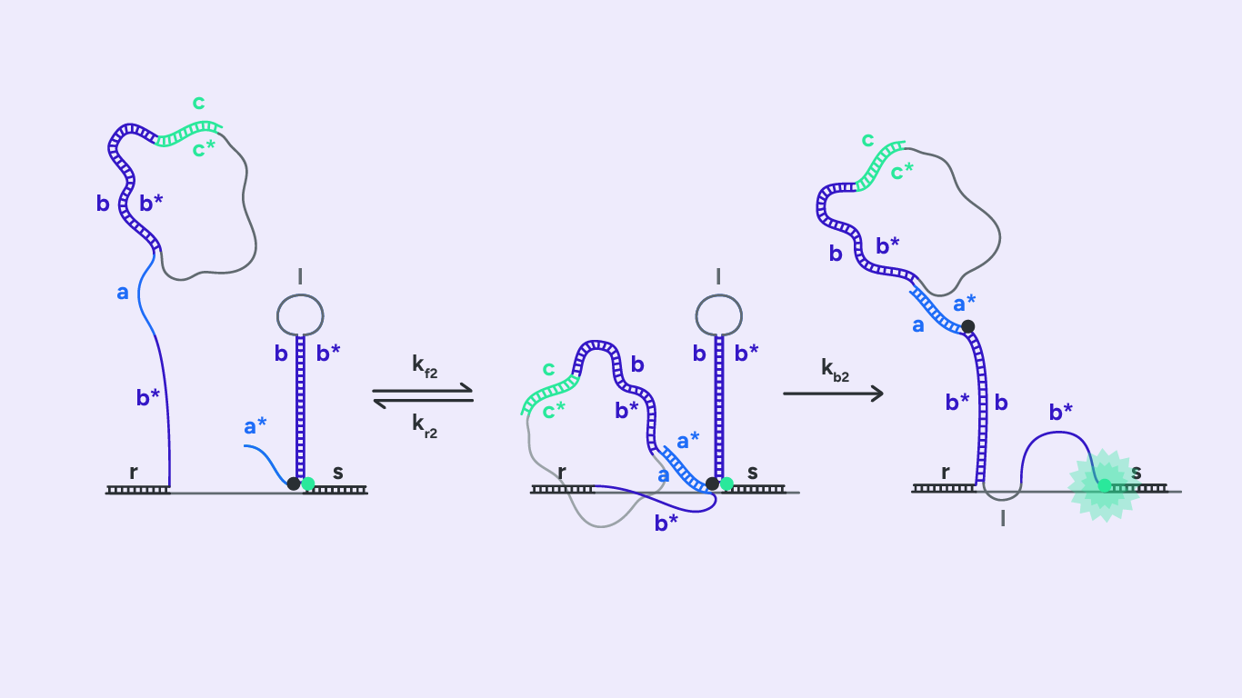
As depicted in Fig.3, H2 also consists of five domains a*, b, a, b*, and r. Initially, H2 forms a stem-loop conformation by hybridizing the two complementary domains, b and b*. The formed loop consists of domain l. Like H1, the H2 hairpin possesses two overhang regions: a toehold domain, a* domain, and an RCA binding domain, s domain. In addition, H2 brings a fluorophore and a quencher. We represent them in Fig3 as a green and a black dot, respectively.

The second toehold reaction is illustrated in Fig.4. Toehold domain a* binds to H1’s complementary domain a. After the toehold invasion, branch migration displacement occurs. The H1 b domain displaces the stem b domain. H2 now exists in an open conformation, which results in the fluorophore diverging from the quencher and emitting fluorescence when excited at the right wavelength.

As in step 1, the rate k_f2 represents the hybridization rate of toehold domain a* to its complement. In addition, the rate k_b2 denotes the rate at which the branch migration junction crosses the middle of the b domain. Finally, k_r2 denotes the rate at which toehold a* frays and dissociates.

k_r2 = k_f2·(2/b)·e^ΔGo(a)/RT [II]

where ΔG^o(a) < 0 is the binding energy between a and its complement, and b the length of b domain.

KinDA: Kinetic DNA strand displacement analyzer

KinDA [2] is a python package that can predict system kinetic and thermodynamic behavior at the sequence level. With KinDA, we can determine if the system as a whole behaves as designed. We tested KinDA through the available Amazon Web Services (AWS) Amazon Machine Image (AMI).

First, the user creates a PIL file that specifies the domains, as described above, stands, and complexes of the DNA strand-displacement system. An example of the user input is the following

#0102533_step1.pil

# Specify all domains
sequence c = CTGTAATCGC : 10
sequence b = TCACTCTGGATTTCTATCAA : 20
sequence a = GACATCTACCAACA : 14
sequence r = CTCATACCATAT : 12
sequence s = TTGCCATGAAAAAGAAAAACTTCCGGATAAGAAAGAAAA : 39

# Specify all strands:
strand h1 = c b a b* r : 76
strand bsj = b* c* : 30
strand rca = r* s : 51

# Specify all predicted complexes:
structure 1 = h1 + rca : .(.)(+).
structure B = bsj : ..
structure 2 = bsj + h1 + rca : .(+)(.)(+).
structure 3 = bsj + h1 + rca : ((+))..(+).

Then, KinDA uses Peppercorn, a reaction enumerator to create the Chain Reaction Network (CRN) at a domain-level. Next, the simulation proceeds with kinetics and thermodynamics analyses at a sequence-level using Multistrand and NUPACK, respectively. Of course, sequence-level interactions may not have direct counterparts in the domain-level system. Hence, KinDA calculates the conformation probability, that is the p-approximation for the sequence-level secondary structure to behave as the domain-level structure, from the fraction of nucleotides that are bound or unbound when both structures share the same ordered strands.

KinDA uses the “first-step reaction model” and separates the reactions into two steps and calculates one constant for each reaction: the initial binding step, with a rate of initiating the reaction, k₁, and the folding trajectory that follows, with the rate of how long it takes to complete, k₂. Errors for k₁and k₂ are determined based on the system parameters. Also, KinDA determines spurious reactions that do not correspond to the predicted behavior and unproductive reactions when reactants and products coincide.

The Simulation

We simulated our two steps as separate reactions. We chose this design because the system categorizes two complexes with the same strand order but different dot-and-bracket notation as a single reactant multiset and calculates the total k₁and k₂. So, we decided to run a simulation for each step and retrieve the individual rate constant. Also, with two simulations, we could decrease the system's complexity to take only a few hours on a t2.micro instance.

We calculated the following rates for the 1st toehold-mediated strand displacement reaction:

k_1(i) : (3.41 ± 0.887) 10⁷
k_2(i) : (2.18 ± 0.576) 10⁷

In this model: k_1(i) = k_f1 [k_b1 / (k_b1+k_r1)] [III], k_2(i) = k_b1 [IV]

From [I] we calculated that k_f1 >>> k_r1, using the value of ΔG_o(c) = -10.88 kcal/mol, as calculated by ViennaRNA. So, we can assume that the toehold domain is long enough so that the dissociation step proceeds slowly relative to the toehold invasion step. Hence, the toehold invasion step determines the rate of the whole reaction.

Then we calculated the following rates for the 2nd toehold-mediated strand displacement reaction:

Following the same process, we proved that the toehold invasion step again determines the rate of the whole reaction.

The results

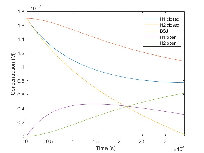
Modifying a MATLAB script provided by our partners, the Thessaloniki_Meta team, we simulated our KinDA results. The plot for hsa_circ_0102533 is depicted in Fig.5. The equations for the simulated reactions are the following:

[H1-closed]/dt = - k_1(i) [H1-closed][BSJ]
[BSJ]/dt = - k_1(i) [H1-closed][BSJ]
[H1-open]/dt = k_1(i) [H1][BSJ] - k_1(ii)[H2-closed][H1-open]
[H2-closed]/dt = - k_1(ii)[H2-closed][H1-open]
[H2-open]/dt = k_1(ii)[H2-closed][H1-open]

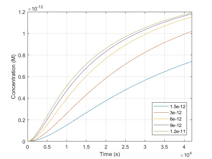
The initial concentrations of [H1-closed] and [H2-closed] in the simulation correspond to H1, and H2 probes hybridized on the linear scaffold in their closed conformation. We run a script using multiple target concentrations, [BSJ]. We used 42.000 sec as our simulation time, the same as the experimental. We observe that [H2-open] increases with time for all given [BSJ] concentrations. Also, [H2-open] maximum concentration increases with [BSJ]. It is crucial because [H2-open] determines the response signal, confirming our laboratory results.

Literature Results

In search engines such as PubMed, we performed the following search: "circular RNA" OR "circular RNA" OR "circRNA" OR "circRNA" AND "lung cancer" AND ("liquid biopsy" OR "biomarker" OR "non-invasive"). We retrieved a total of 119 results that we sorted by title and abstract into the following categories:

• Articles employing the use of a circRNA as a diagnostic biomarker for lung cancer
• Articles employing the use of a circRNA as a prognostic biomarker for lung cancer
• Articles regarding the function of a circRNA in the initiation and progression of lung cancer
• Articles that examine the role of a circRNA in the drug resistance shown by lung cancer patients
• Review summarizing the role of circRNAs in lung cancer

We rejected articles about other types of cancer. We further studied the articles in the first category to select the biomarkers. Articles belonging to the latter category were studied to establish the necessary knowledge regarding the role of circRNAs, specifically for the type of cancer in question.

We categorized circRNAs reported in the first category articles as potential targets according to their characteristics. Then, we selected the studies conducted on blood samples from patients with NSCLC. The studies should have had sufficient samples of patients and healthy volunteers and included patients in the early stages of the disease. Articles regarding circRNAs that are potential targets for NSCLC subtypes, such as lung adenocarcinoma, were not rejected. However, CircRNAs detected exclusively in cancer tissues and circRNAs detected in plasma exosomes and not directly in patient plasma were discarded.

From the total of 119 search results, we finally selected ten articles that concern the expression of 11 circRNAs, nine were found to be abnormally increased, and the remaining two abnormally decreased in the plasma of NSCLC patients. The publication dates of the articles start from July 2017, with the latest reaching January 2022. Then, we tabulated the characteristics of each selected study/circRNA for easier comparison. These tables included:

• the name of the circular RNA,
• the type of lung cancer they have and,
• the number of patients and healthy volunteers who took part in the study,
• the biological material (e.g., plasma, serum, tissues, cell cultures),
• the detection method (e.g., RT-PCR),
• the specificity and sensitivity values calculated for the biomarker, and other results.

Databases for circular RNAs

After finding the 11 targets, we deemed it necessary to narrow our panel to only three circRNAs further to be detected at the laboratory level so that the experiments could meet the time frame of the competition. Initially, we compared each biomarker's sensitivity and specificity values ​​and their detection in the early stages of the disease.

However, literature data were insufficient to make the optimal choice, so more information about the target molecules was searched in databases. The bases concern exclusively circRNAs and those used are the following: circBase, circBank, circAtlas, circRNADb [3], [4], [5], [6]. The information collected concerns the number of nucleotides of the circRNAs, the target gene, their sequence, and their expression in cell lines. As we had decided to start by testing the diagnostic ability of LDN on circRNAs isolated from lung cancer cell lines, the expression profile of these circRNAs in cell lines was examined using information collected from the databases [7], [8], [9].

Also, we embedded the use of Cancer-specific circRNAs database CSCD [10], a database that collects available RNA sequencing datasets from 87 cancer cell line samples. Using the genomic coordinates from circBank, we output information, including expression in normal and lung cancer cell lines, ratios (circRNA/linear gene), cellular location, prediction algorithm, and abundance. Since we had A549 and H1299 cell lines available in the laboratory, RNAs aberrantly expressed in them were preferred. We compared these data with the expression in normal cell lines or lines of other cancer types. Targets that were unique to non-small cell cancer were preferred. We discarded circRNAs that could not complete crossover between the different sources.

The three final targets were hsa_circ_0070354, hsa_circ_0102533 and hsa_circ_0005962.

GEO datasets

We performed a search using the Gene Expression Omnibus (GEO) [11] dataset using "lung cancer" OR "lung tumor" AND "circRNA" and a second search using "lung cancer" AND ("plasma circRNA" or "blood circRNA" or "serum circRNA").

Unfortunately, we reached results (GSE101586, GSE101684, and GSE112214) with samples from adenocarcinoma tissues, not blood samples. In addition, these studies included 3-5 patients and 3-5 healthy participants, which is insufficient for conducting Bioinformatic analysis. This insufficiency of results only confirms that circRNA research is in its initial phase and arises from the fact that non-polyadenylated (poly(A)−) transcripts, including circular RNAs (circRNAs), skew quantification in multiple techniques, such as Next Generation Sequencing (NGS). To detect our targets, we must enrich certain transcript types prior to sequencing to focus on the most relevant populations (for example, separation of poly(A)+ and poly(A)− RNA populations). These enrichment approaches can simplify bioinformatic analyses and enhance statistical power [36],[37]. Unfortunately, circRNAs have not been researched enough for these methods to be applied to blood samples of every disease type. With syn-PNOIA, we propose a tool for detecting circRNAs to bring these biomarkers into focus.

Secondary structure prediction

After we selected our three circRNA biomarkers and derived their sequences in the previously mentioned databases, we proceeded with the H1 and H2 probes design. The process is schematically represented in Fig.7

The back-splice junction (BSJ) site is a specific point for each circRNA target, and it separates them from their linear isoforms, RNAs originating from the same gene. So, we considered it better to design our Nanostructure based on the ability to detect this sequence. Initially, we chose 15 bases upstream and 15 downstream of the BSJ site as the target sequence.

Based on the BSJ sequence, we created the H1 probe to consist of the following domains:

• A domain complementary to the BSJ sequence to "identify" the target circRNA among the various RNAs present in the sample (1)
• The loop domain (2)
• A domain complementary to 20 bases of sequence (1) to create a 20-base hairpin stem (3)
• A domain complementary to the RCA product (4)

We created the H2 probe accordingly:

• A domain complementary to the RCA product (5),
• A domain complementary to sequences (2) and (3) that is responsible for the hybridization of the two probes (6),
• A domain complementary to 20 bases of sequence (6) to create a 20-base hairpin stem (7)
• The loop domain (8)

Taking the above into consideration, the first step of our Model design was to validate if the designed H1 and H2 probe sequences had the desired hairpin formation and how they interact with the linear DNA backbone when forming the LDN to determine whether the result is structurally acceptable. Using the NUPACK software suite [12], which uses SantaLucia's nearest neighbor model [13], we analyzed our structures at 37.0 ^oC and 1.05 M salt concentration (1.0M Na⁺ and 0.05M Mg⁺²) to replicate our reaction conditions as close to reality as possible.

We were satisfied that our system conformed to the desired structure while keeping theGibbs free energy (ΔG) energy levels low, proving a thermodynamically stable system. However, our original selection of 15 bases both upstream and downstream, respectively, do not invariably achieve the desired result. At this point, a question was presented to us. Was there a better H1 and H2 probes combination than the one we had chosen?

As you can imagine, creating each structure by hand is a very tedious and time-consuming process. Therefore, we automated our design using a python script that creates and simulates all possible combinations of LDNs that can occur given the mature circRNA sequence. You can view our ldn_generator.py script by clicking the interactive button below. See more details on the design behind the ldn_generator.py script on the Contribution page. Finally, all nucleic acid secondary structures are represented in the dot-parens-plus notation.

Unexpectedly, we observed no vast difference in ΔG between the various H1 and H2 probes and the LDN, proving our initial design was thermodynamically favored. Structural differences between the possible structures, self hybridization of the one dangling end to the other and the presence of secondary loops might hinder the LDN’s ability to function correctly at 37 ^oC.

CircRNA secondary structure

A necessary component to understanding our system and progressing our Modeling work is the illustration of how the circular RNAs appeared to be in space. Hence, we used the ViennaRNA Web services, particularly the RNAfold server, a gold standard in RNA 2D visualization [14], [15]. By importing the mature circRNA sequence and selecting the "assume RNA molecule to be circular" option under the advanced options menu, we generated the secondary structure for the circRNA targets.

In the output, two different predictions are depicted: the Minimum Free Energy structure (MFE) and the Centroid structure, which represent the equilibrium ensemble differently. For the next steps of our Model, we used the MFE structure, depicted in Fig.8.The circRNAs had the following Gibbs free energy:

Hsa_circ_0070354: ΔG = -105.60 kcal/mol

Hsa_circ_0102533: ΔG = -222.10 kcal/mol

Hsa_circ_0005962: ΔG = -79.90 kcal/mol

Tertiary structure prediction and Molecular Dynamics

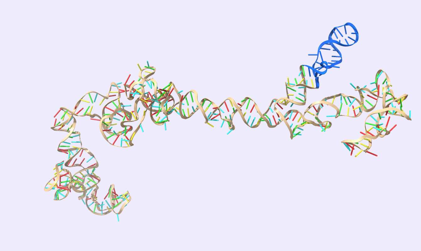
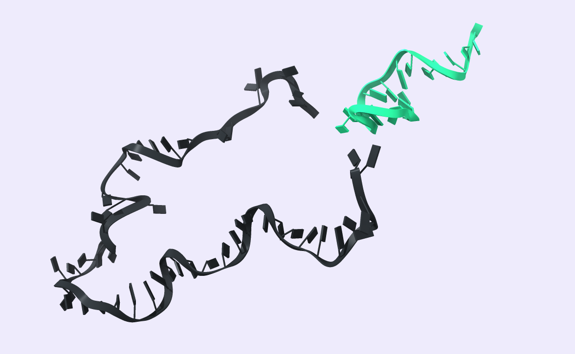
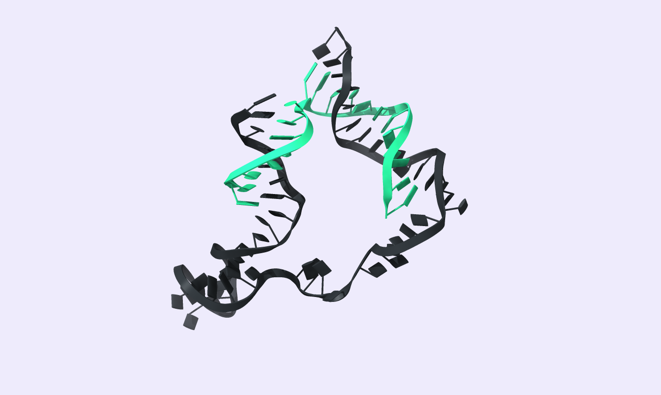
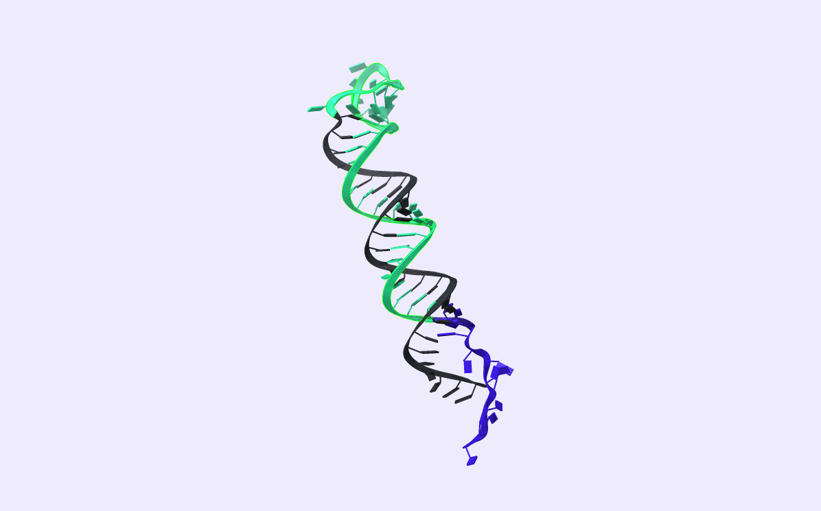
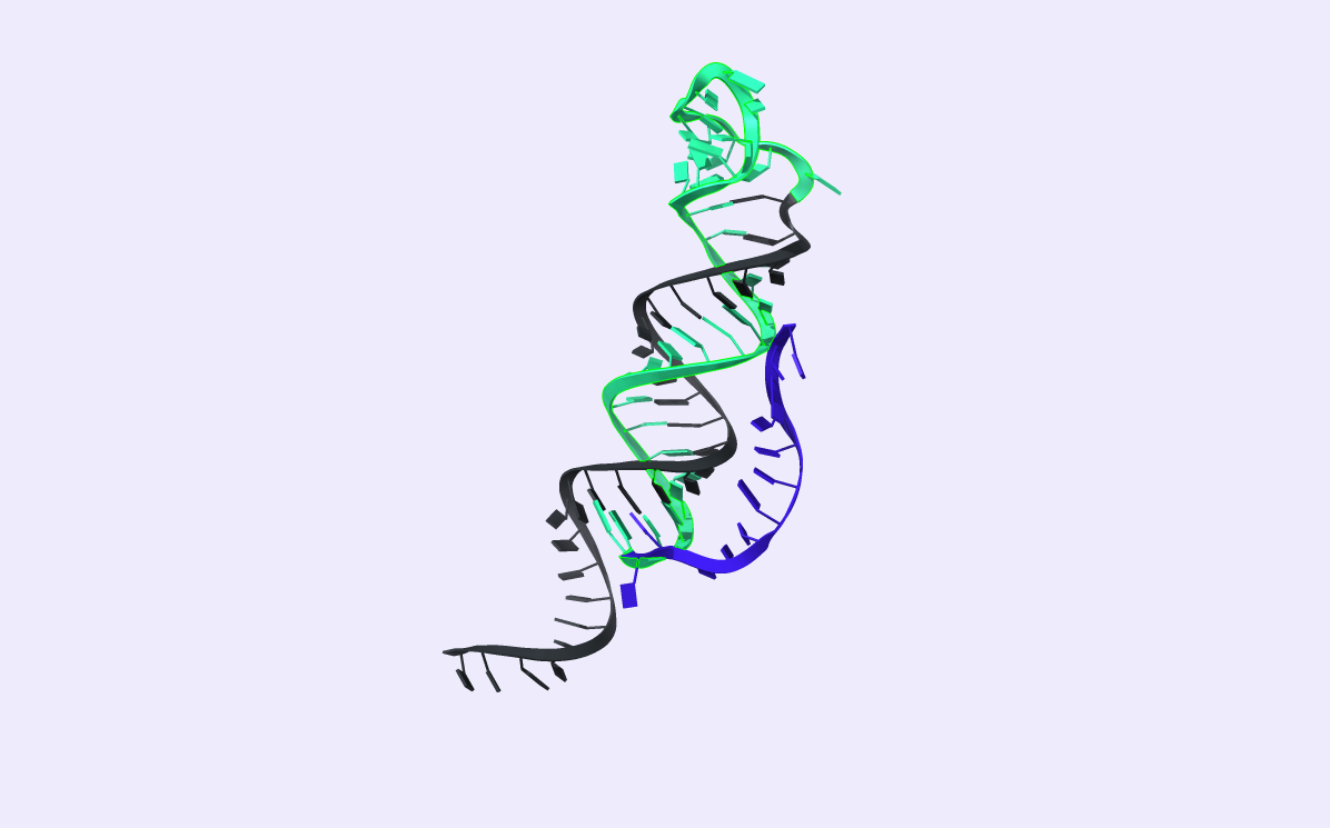
Two methods were implemented, one to model the structure of the circular RNAs and one to model the LDN system's components. Following the secondary structure prediction and our understanding that circular RNAs are far from a circle, we aimed to model their tertiary structure in order to identify where the back splice junction domain is located. That proves to be a valuable point when designing our structure, because if the BSJ site is located in a place where steric hindrance occurs it would be difficult to be accessed by our Nanostructure. As a result the detection reaction would take longer than expected or even not accomplished at all.

CircRNAs were modeled using 3DRNA/DNA web services [16], which functions as a comparative modeling method and an ab initio method combining user-defined data and already characterized nucleic acid segments to obtain the best possible tertiary structure. By importing the mature circRNA sequence and the corresponding secondary structure obtained in the previous step, the server follows a pipeline of assembling the smallest secondary elements (SSEs) containing stem (helix), hairpin loop, internal loop, bulge loop, pseudoknot loop, and junction loop, from already characterized RNA PDB files and optimizing the structure with Monte Carlo simulations. After the simulation, multiple models are depicted, all scored by a 3dRNA score acting as a method to evaluate distance and torsion angle functions of the structure, where a lower value corresponds to a better structure. Hsa_circ_0070354 scored 26.3831, hsa_circ_0102533 scored 26.5516 and hsa_circ_0005962 scored 26.7353, values low enough considering their complex structure.

After comparing the output to the original secondary structure, we obtain the 3D structure of choice. We visualized the circRNA 3D structure using UCSF Chimera X [17] and Visual Molecular Dynamics (VMD) [18], [19]. These next-generation molecular visualization programs provide a command line and a Graphical User Interface. By the interactive side panel, the BSJ site is selected, and it is differentiated by blue color from the remaining structure. In Fig.9, all three circRNA targets are depicted providing an easy-to-access BSJ site.

Since there is not an already characterized structure of the designed Nanostructure, it is necessary to follow a different modeling approach. As described carefully on the Project Description page, LDN acts as a polymer of specific repeats of H1 and H2 probe domains. In order to simplify our system and after various Human Practices discussions, we decided that it is better to model one of the multiple repeating structures and to assume that the remaining Nanostructure acts in the same way.

Our first step was to monitor the conformation of the H1 and H2 probes separately by modeling. We utilized a coarse-grained DNA model, called oxDNA. OxDNA is a simulation code designed to implement Monte Carlo and Molecular Dynamics to analyze DNA and RNA structures, supporting simulations on both CPU [20] and Nvidia CUDA backends [21]. The Model treats DNA as a string of rigid nucleotides, which interact through potentials that depend on the position and orientation of the nucleotides, leading to faster simulations than if an all-atomistic approach was followed. In addition, it treats each sugar-phosphate backbone and each nitrogenous base as a single entity, but with specific electrostatic properties. Hydrogen bonds occur between complementary bases when they are anti-aligned, forming double helical structures [22]. Three different simulation techniques can be used with oxDNA [23]:

• Metropolis Monte Carlo (MC) simulations sample a Boltzmann distribution to propose nucleotide configurational moves.
• Virtual Move Monte Carlo (VMMC) simulations generate co-moving nucleotide clusters to assess pairwise interactions, circumventing MC simulation's drawbacks.
• Molecular Dynamics (MD) simulations according to which molecule moves are predicted based on Newton's laws of motion.

We used the VMMC model for our simulations as, in systems with less than 100 nucleotides, equilibration is reached faster with VMMC than with MD.

We used oxDNA for three essential simulations:

• Hybridization of RCA primer to the linear phosphorylated template
• Hairpin probe H1 and H2 formation
• Linear DNA Nanostructure construction

Initially, organizing the expected simulation steps and results is very important. Therefore, initial input file preparation is crucial for Molecular Dynamics simulations. OxDNA uses two separate files to characterize a sequence, a topology (.top) file and a configuration (.conf) file. The .top file stores the intra-strand fixed topology in the order the nucleotides are depicted. The .conf file contains the current timestep, the length of the simulation box's sides, and the total, potential, and kinetic energies. On the configuration file after an original header, information about every single nucleotide, such as the velocity, is depicted. More information about the input files is mentioned in the oxDNA documentation [24]. We must consider that due to legacy reasons, the simulation code prefers structures to be listed in reverse direction (3' → 5'). Using an online converter [25], we prepared all the input sequences and transferred them to a .txt file in the correct order. Using the generate-sa.py script provided with the oxDNA pack, we can generate the structure input files based on the original .txt file. Note that the simulation box should have box sides at least as big as the largest sequence in the .txt file.

As output files we are expecting three different file types:

• A trajectory (.dat) depicting how our system changes conformations with each timestep.
• A last configuration (.conf) file to be used for the conversion of the oxDNA files to all-atomic Protein Data Bank (.pdb) structures.
• An energy file (.dat), to be plotted so we can estimate if our system has reached equilibration.

The next step is to prepare the input file for the simulation process. The user defines the options in a text file with a key = value style. We set the simulation parameters to be as suitable and compatible as possible to our experimental design. Before each simulation we performed a standard relaxation procedure, consisting of :

• 10³ steps of MC simulations on a CPU, followed by
• 10⁶ steps of an MD relaxation on CUDA with a maximum-value of the cutoff for the backbone potential

The oxDNA2 model [26] was used, since it allows DNA to be studied with salt concentrations, and sequence-specific parameters were applied. The temperature and salt concentration were set according to each experiment. You can view all our input options in their corresponding files on our GitHub Page. The visualization of the output was achieved using oxView [27], a web-service that provides the ability for oxDNA models to be dynamically represented through their initial .top file and the output trajectory or last configuration files.

Primer hybridization to phosphorylated template

First step to our project was the creation of the circular DNA template, by hybridization of RCA primer to the phosphorylated template. Modeling that structure proved to be a simple task, following the oxDNA pipeline described earlier, we just had to incorporate one more aspect, that of Mutual Traps. If we let our system reach equilibration on its own, it would take at least 108 timesteps for a simple oligonucleotide hybridization, amounting to time-consuming simulations. Mutual Traps act as time-sustained external forces bringing user-defined complementary and anti-aligned nucleotides closer. See more details in the Contribution page on how to orchestrate a Mutual By incorporating these forces in the first and last nucleotide of the primer and their complementary nucleotides in the template sequence we are able to reach equilibration obtaining the desired structure.Simulation was run with a temperature set to 25 ^oC. In Fig.10 the initial and equilibrated tertiary structures are presented before and after oxDNA simulation.

Probe formation

One of the primary uses of oxDNA, apart from origami DNA structure visualization, is hairpin formation. We obtained the trajectories, tertiary structures, and energy files for each of the hairpin probes used in our project. By setting the temperature to 25 ^oC. You can observe that each probe has the expected loop structure and the two hanging tails, one for target detection and one for binding to the DNA backbone. Equilibration was achieved in 10⁸ steps.

Nanostructure formation

Importing the modeled probe tertiary structures and the RCA domain, in oxView using the topology and last configuration files, we exported the image in oxDNA files, to be used for the next simulation. We set the temperature to 37.0 ^oC and salt concentration to 1.05M, using the corresponding Mutual Traps, and in just 10⁶ time-steps the Nanostructure was formed retaining the designed structure.

In order to use these results for further simulations, conversion to all-atomistic PDB files is necessary. First step was to install Python2 to WSL2 since most of the legacy utility scripts provided with oxDNA are written in Python2. Using the supplied convert_to_atomic.py script we obtained the desired structures. Upon visualization of the generated PDB files, we observed that in VMD bond breaks were apparent, whereas in ChimeraX the desired structure was depicted. After hours of trying to figure out if we had done something wrong during the simulation or during the .pdb file conversion, we found a discussion page in the oxDNA forum pointing out that this is a common problem presented when converting coarse-grained models to all-atomistic ones. So we decided to continue with the generated .pdb files.

Stability analysis

Two different components were examined for their stability, the circular DNA template and its binding to phi29 DNA Polymerase. Importing the PDB files obtained from oxDNA, to GROMACS we followed the steps described in the Contribution page in order to minimize the system and follow a standard MD stability protocol. In the trajectory produced for 1ns the circular DNA template retained its structure, with bonds breaking and forming again.

Protein-DNA interactions

Two interactions were studied: The T4 DNA ligase binding to the circular DNA template and the interaction between phi29 DNA polymerase and the template. The first step was to do a docking analysis on the desired complexes. PDB files for the T4 DNA ligase and the phi29 DNA polymerase were obtained from the PDB server as complexes with target DNA. Using VMD, we exported the protein structure as a new PDB file to be used for docking. Using the HDOCK web server [35], we got:

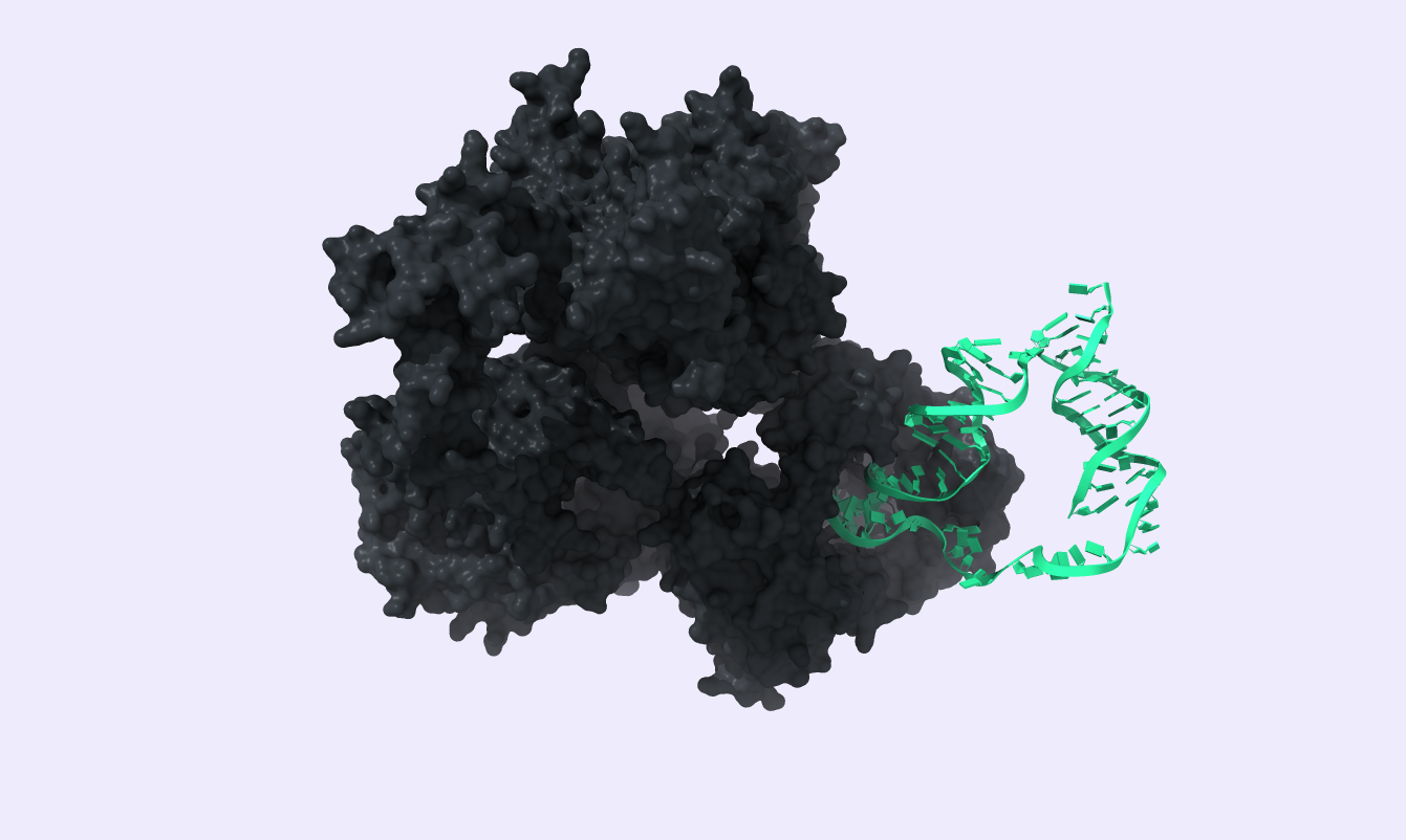
After docking the DNA template to phi29 DNA polymerase, we proceeded to a Molecular Dynamics analysis to verify the created complex's stability. For this protein-DNA complex, the Molecular Dynamic simulation parameters are specified above. A 1ns simulation was produced with the trajectory displayed below, proving the desired stability of our complex, indicating that we should further develop our Modeling work.